
In my previous blog entry I showed the large discrepancies in the magnitude of reconstructed paleo climate estimates between the ice core and ocean sediment proxies based on oxygen isotope ratio analysis. I made two sets of adjustments to the proxy data to bring them into better alignment – a high grouping and a low grouping. The high grouping shows higher glacial period temperatures and the low grouping lower glacial period temperatures.
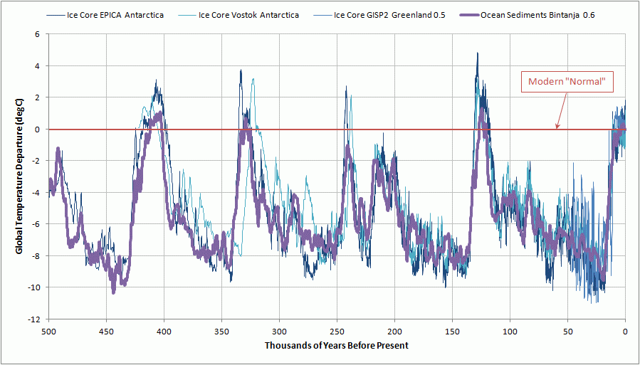
In the high grouping I multiplied the Greenland GISP 2 ice core analysis by 0.5 and the Bintanja ocean sediment analysis by 0.6 to reduce their offsets from our modern “normal” climate reference and thus bring them into better alignment with the Vostok and EPICA ice core analyses from Antarctica, as shown below (click to enlarge).

A comparison of adjusted climate reconstructions from a composite of many ocean sediment cores (Bintanja) versus three different ice core reconstructions (Greenland GISP2 and Vostok and EPICA from Antarctica). The ice core reconstructions have been adjusted by the factor indicated to better match the ocean sediment reconstruction.
For the low grouping I increased the offsets from the modern “normal” climate reference by multiplying the Vostok and EPICA ice core analyses by 1.6 to bring them into better alignment with the Bintanja ocean sediment analysis. In this case I also multiplied the GISP 2 analysis by 0.9 to bring it into better alignment with the Bintanja analysis. The result is shown below (click to enlarge).
A comparison of adjusted climate reconstructions from a composite of many ocean sediment cores (Bintanja) versus three different ice core reconstructions (Greenland GISP2 and Vostok and EPICA from Antarctica). The composite ocean core reconstruction and Greenland GISP2 ice core reconstruction have been adjusted by the factor indicated to better match the Antarctica Vostok and EPICA ice core reconstructions.
Notice that even though the patterns are very similar between the two adjusted groupings, the temperature scale is much different. The high grouping shows the lowest glacial period global temperatures about 8 to 10 degrees Centigrade (C) below our modern “normal” while the low grouping shows global temperatures about 12C to 18C below. Likewise, the high grouping shows maximum interglacial warm period temperatures as much as 1C to 4C above our modern “normal” while the low grouping shows peak interglacial temperatures 2C to 8C above our modern “normal”.
I find the high grouping to be more aesthetically appealing because it doesn’t look quite as noisy, but I’m not sure which of these two groupings might be more accurate. The differences between them reenforce the uncertainty of the magnitude of past global climate variations. The timing of major events is remarkably similar between these proxies, although that might result from similar methods in relating the proxie measurements to a time scale for the reconstruction.
I my next post I will make a paleo climate persistence forecast based on the EPICA ice core analyses by comparing our current interglacial period with the previous four interglacials.
